The math behind digital sampling and filtering is fascinating, complex, and full of arcane terms like Nyquist frequency. But I'm barely a good enough mathematician to understand it, let alone try to explain it here! This post is my attempt to describe aliasing as it applies to computer graphics via overgeneralized hand waving.
Most of the important operations involved in rendering graphics can be boiled down to digitally sampling a signal. If this phrase is new to you, don't panic! A signal just means a value that changes as you move around some coordinate space (which can be 1D, 2D, or occasionally 3D or more). Common types of signal used in graphics are:
Signals can sometimes be described by a mathematical equation, but they are more commonly represented as a series of digital samples, ie. an array which stores the value of the signal for many different coordinate locations.
<digression>
People often claim that the real world uses continuously varying analog signals, but when you get down to the quantum level it is actually all digital samples! Subatomic particles are entirely discrete. Photons are either there or not there, so the brightness of a light can never involve a fractional number of photons. Things only appear continuous because these particles are so small. Reality is pixelated, just at a ridiculously high resolution :-)
</digression>
Sampling occurs whenever we wish to transform one signal into another, for instance:
Although the implementation tends to be heavily optimized, all forms of sampling work basically the same way:
Easy, right? But this basic operation is where pretty much every kind of aliasing comes from.
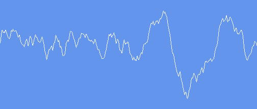
Example time. Consider this 1D signal, stored as an array of 512 digital values:
Let's convert this signal to an array of just 64 values, by taking evenly spaced samples every 8 entries through the original. Note that there is no requirement for our samples to be evenly spaced. That makes it easy to visualize, but if we were for instance mapping a texture onto the side of an object rendered with a 3D perspective view, the relationship between input and output samples could be a more complex curve function.
This resampling produces a new signal with the same basic shape as the original, but less detail:
It looks ugly and blocky, but that is actually a made-up problem caused by the fact that after shrinking my 512 sample signal to just 64 samples, I scaled back up to 512 before displaying the above image. If I displayed the downsampled signal at its native 64 pixel width, there would be no such blockiness.
If I did for some reason need to shrink the signal to 64 samples and then scale back up to 512, I could do that scaling by interpolating between values rather than just repeating them. This is called linear filtering (the previous example used point sampling) and it produces an image that looks pleasingly similar to our original, albeit with less fine detail:
Here's where it gets interesting. Look what happens if we reduce the output signal to just 16 samples:
Then 8:
7:
And finally 6:
Whoah! How come 8 samples has a dip followed by peak toward the right of the signal, but the 7 sample version is almost flat, while the 6 sample version has a peak followed by dip, almost the exact opposite of the 8 sample version?
The problem is that when we are taking so few samples, there just aren't enough values to accurately represent the shape of the original signal. It ends up being basically random where in the signal these samples happen to be taken, so our output signal can change dramatically when we make even small adjustments to how we are sampling it. When reducing a signal to dramatically fewer samples than were present in the original, the result tends to be meaningless noise.
Aliasing can be a problem even when you are not dramatically reducing the number of samples. Consider our original 512 sample signal, which includes a lot of small, high frequency jitter. Then consider the 64 sample version, which has the same basic shape but without that fine detail. This looks fine as a still image, but what if were to animate it, perhaps sliding the curve gradually sideways? Now each frame of the animation will be sampling from slightly different locations in the original signal. One frame our sample location may randomly happen to be at the top of one of those little jitters, then the next frame it could be at the bottom. The result is that our output signal randomly jitters up and down, in addition to sliding sideways!
This is a common characteristic of aliasing problems. In extreme cases they can make even static images look bad, but more often, subtle aliasing may look fine when stationary yet will flicker or shimmer whenever the object or camera moves.
Fun way to see an extreme example of this in action:
Up next: ways to avoid aliasing when resampling a signal.